4 Overview

An example analysis that very briefly demonstrates some of the tasks that we’ll tackle during the workshop.

4.1 Preparation

Make sure we have the packages we need from CRAN:

pkgs <- c("dplyr", "ncdf4", "raster", "remotes", "robis", "worrms")
pkgs <- setdiff(pkgs, installed.packages()[, 1])
if (length(pkgs) > 0) install.packages(pkgs)

library(dplyr)

And from GitHub:

## packages with required minimum version
pkgs <- c("SCAR/antanym" = NA, "AustralianAntarcticDivision/blueant" = NA,
          "AustralianAntarcticDivision/SOmap" =  "0.5.1")
for (pkg in names(pkgs)) {
    if (!basename(pkg) %in% installed.packages()[, 1] ||
        (!is.na(pkgs[[pkg]]) && packageVersion(basename(pkg)) < pkgs[[pkg]])) {
        remotes::install_github(pkg)
    }
}

4.2 Taxonomy

library(worrms)

my_species <- "Euphausia crystallorophias"
tax <- wm_records_names(name = my_species)
tax

## [[1]]
## # A tibble: 1 x 27
##   AphiaID url                                                          
##     <int> <chr>                                                        
## 1  236216 http://www.marinespecies.org/aphia.php?p=taxdetails&id=236216
##   scientificname             authority               status  
##   <chr>                      <chr>                   <chr>   
## 1 Euphausia crystallorophias Holt & Tattersall, 1906 accepted
##   unacceptreason taxonRankID rank    valid_AphiaID
##   <lgl>                <int> <chr>           <int>
## 1 NA                     220 Species        236216
##   valid_name                 valid_authority         parentNameUsageID
##   <chr>                      <chr>                               <int>
## 1 Euphausia crystallorophias Holt & Tattersall, 1906            110673
##   kingdom  phylum     class        order        family       genus    
##   <chr>    <chr>      <chr>        <chr>        <chr>        <chr>    
## 1 Animalia Arthropoda Malacostraca Euphausiacea Euphausiidae Euphausia
##   citation                                                                 
##   <chr>                                                                    
## 1 Siegel, V. (Ed) (2019). World Euphausiacea Database. Euphausia crystallo~
##   lsid                                      isMarine isBrackish
##   <chr>                                        <int> <lgl>     
## 1 urn:lsid:marinespecies.org:taxname:236216        1 NA        
##   isFreshwater isTerrestrial isExtinct match_type modified                
##   <lgl>        <lgl>         <lgl>     <chr>      <chr>                   
## 1 NA           NA            NA        exact      2010-03-02T17:11:18.233Z

## the Aphia ID (taxonomic ID) of our species
my_aphia_id <- tax[[1]]$valid_AphiaID

4.3 Occurrences

Get all data from the Antarctic Euphausiacea occurence data from “German Antarctic Marine Living Resources” (GAMLR) Expeditions data set:

library(robis)
x <- occurrence(datasetid = "cb16377b-56a8-4d95-802d-4eec02466773")

Plot the complete distribution of samples in black, and Euphausia crystallorophias in green:

library(SOmap)
SOmap_auto(x$decimalLongitude, x$decimalLatitude, input_lines = FALSE, pcol = "black", pcex = 0.2)
with(x %>% dplyr::filter(aphiaID == my_aphia_id), 
     SOplot(decimalLongitude, decimalLatitude, pch = 19, cex = 0.2, col = "green"))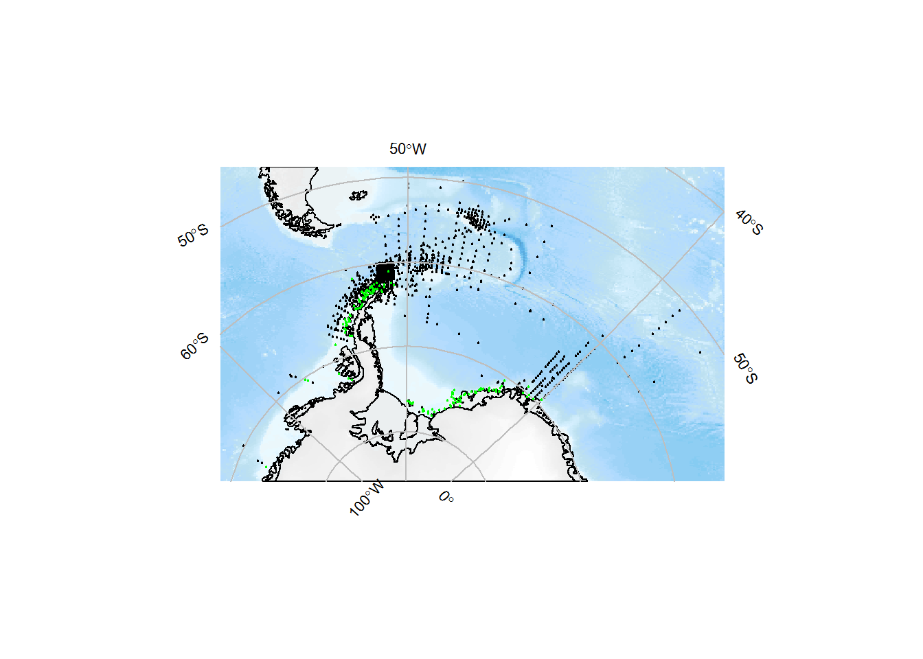

Or as a polar stereo map:

basemap <- SOmap(trim = ceiling(max(x$decimalLatitude))+1, bathy_legend = FALSE)
plot(basemap)
SOplot(x$decimalLongitude, x$decimalLatitude, pch = 19, cex = 0.2, col = "black")
with(x %>% dplyr::filter(aphiaID == my_aphia_id), 
     SOplot(decimalLongitude, decimalLatitude, pch = 19, cex = 0.2, col = "green"))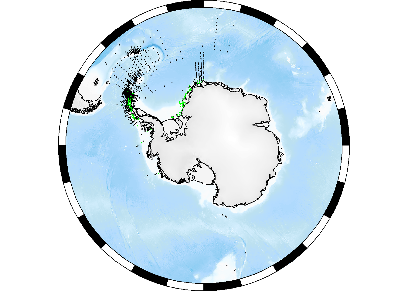

We’re going to fit a species (presence/absence) distribution model, so first let’s reorganise our data into presence/absence by sampling site:

xfit <- x %>% dplyr::rename(lon = "decimalLongitude", lat = "decimalLatitude") %>%
    group_by(lon, lat) %>%
    dplyr::summarize(present = any(my_aphia_id %in% aphiaID))

4.4 Environmental data

library(blueant)
## put the data into a temporary directory
my_data_directory <- tempdir()

## the data source we want
data_source <- sources_sdm("Southern Ocean marine environmental data")

## fetch the data
status <- bb_get(data_source, local_file_root = my_data_directory, verbose = TRUE)

## 
## Tue Oct 22 13:14:33 2019
## Synchronizing dataset: Southern Ocean marine environmental data
## --------------------------------------------------------------------------------------------
## 
##  this dataset path is: C:\Users\ben_ray\AppData\Local\Temp\RtmpE3w3qi/services.aad.gov.au/public/datasets/science/environmental_layers
##  downloading file 1 of 1: http://services.aad.gov.au/public/datasets/science/environmental_layers/POC_2005_2012_ampli.nc ...  done.
##  downloading file 1 of 1: http://services.aad.gov.au/public/datasets/science/environmental_layers/POC_2005_2012_max.nc ...  done.
##  downloading file 1 of 1: http://services.aad.gov.au/public/datasets/science/environmental_layers/POC_2005_2012_mean.nc ...  done.
##  downloading file 1 of 1: http://services.aad.gov.au/public/datasets/science/environmental_layers/POC_2005_2012_min.nc ...  done.
##  downloading file 1 of 1: http://services.aad.gov.au/public/datasets/science/environmental_layers/POC_2005_2012_sd.nc ...  done.
##  downloading file 1 of 1: http://services.aad.gov.au/public/datasets/science/environmental_layers/chla_ampli_alltime_2005_2012.nc ...  done.
##  downloading file 1 of 1: http://services.aad.gov.au/public/datasets/science/environmental_layers/chla_max_alltime_2005_2012.nc ...  done.
##  downloading file 1 of 1: http://services.aad.gov.au/public/datasets/science/environmental_layers/chla_mean_alltime_2005_2012.nc ...  done.
##  downloading file 1 of 1: http://services.aad.gov.au/public/datasets/science/environmental_layers/chla_min_alltime_2005_2012.nc ...  done.
##  downloading file 1 of 1: http://services.aad.gov.au/public/datasets/science/environmental_layers/chla_sd_alltime_2005_2012.nc ...  done.
##  downloading file 1 of 1: http://services.aad.gov.au/public/datasets/science/environmental_layers/depth.nc ...  done.
##  downloading file 1 of 1: http://services.aad.gov.au/public/datasets/science/environmental_layers/distance_antarctica.nc ...  done.
##  downloading file 1 of 1: http://services.aad.gov.au/public/datasets/science/environmental_layers/distance_canyon.nc ...  done.
##  downloading file 1 of 1: http://services.aad.gov.au/public/datasets/science/environmental_layers/distance_max_ice_edge.nc ...  done.
##  downloading file 1 of 1: http://services.aad.gov.au/public/datasets/science/environmental_layers/distance_shelf.nc ...  done.
##  downloading file 1 of 1: http://services.aad.gov.au/public/datasets/science/environmental_layers/extreme_event_max_chl_2005_2012_ampli.nc ...  done.
##  downloading file 1 of 1: http://services.aad.gov.au/public/datasets/science/environmental_layers/extreme_event_max_chl_2005_2012_max.nc ...  done.
##  downloading file 1 of 1: http://services.aad.gov.au/public/datasets/science/environmental_layers/extreme_event_max_chl_2005_2012_mean.nc ...  done.
##  downloading file 1 of 1: http://services.aad.gov.au/public/datasets/science/environmental_layers/extreme_event_max_chl_2005_2012_min.nc ...  done.
##  downloading file 1 of 1: http://services.aad.gov.au/public/datasets/science/environmental_layers/extreme_event_max_sali_2005_2012_nb.nc ...  done.
##  downloading file 1 of 1: http://services.aad.gov.au/public/datasets/science/environmental_layers/extreme_event_max_temp_2005_2012_nb.nc ...  done.
##  downloading file 1 of 1: http://services.aad.gov.au/public/datasets/science/environmental_layers/extreme_event_min_chl_2005_2012_ampli.nc ...  done.
##  downloading file 1 of 1: http://services.aad.gov.au/public/datasets/science/environmental_layers/extreme_event_min_chl_2005_2012_max.nc ...  done.
##  downloading file 1 of 1: http://services.aad.gov.au/public/datasets/science/environmental_layers/extreme_event_min_chl_2005_2012_mean.nc ...  done.
##  downloading file 1 of 1: http://services.aad.gov.au/public/datasets/science/environmental_layers/extreme_event_min_chl_2005_2012_min.nc ...  done.
##  downloading file 1 of 1: http://services.aad.gov.au/public/datasets/science/environmental_layers/extreme_event_min_oxy_1955_2012_nb.nc ...  done.
##  downloading file 1 of 1: http://services.aad.gov.au/public/datasets/science/environmental_layers/extreme_event_min_sali_2005_2012_nb.nc ...  done.
##  downloading file 1 of 1: http://services.aad.gov.au/public/datasets/science/environmental_layers/extreme_event_min_temp_2005_2012_nb.nc ...  done.
##  downloading file 1 of 1: http://services.aad.gov.au/public/datasets/science/environmental_layers/geomorphology.nc ...  done.
##  downloading file 1 of 1: http://services.aad.gov.au/public/datasets/science/environmental_layers/ice_cover_max.nc ...  done.
##  downloading file 1 of 1: http://services.aad.gov.au/public/datasets/science/environmental_layers/ice_cover_mean.nc ...  done.
##  downloading file 1 of 1: http://services.aad.gov.au/public/datasets/science/environmental_layers/ice_cover_min.nc ...  done.
##  downloading file 1 of 1: http://services.aad.gov.au/public/datasets/science/environmental_layers/ice_cover_range.nc ...  done.
##  downloading file 1 of 1: http://services.aad.gov.au/public/datasets/science/environmental_layers/ice_thickness_max.nc ...  done.
##  downloading file 1 of 1: http://services.aad.gov.au/public/datasets/science/environmental_layers/ice_thickness_mean.nc ...  done.
##  downloading file 1 of 1: http://services.aad.gov.au/public/datasets/science/environmental_layers/ice_thickness_min.nc ...  done.
##  downloading file 1 of 1: http://services.aad.gov.au/public/datasets/science/environmental_layers/ice_thickness_range.nc ...  done.
##  downloading file 1 of 1: http://services.aad.gov.au/public/datasets/science/environmental_layers/metadata_details2.csv ...  done.
##  downloading file 1 of 1: http://services.aad.gov.au/public/datasets/science/environmental_layers/mixed_layer_depth.nc ...  done.
##  downloading file 1 of 1: http://services.aad.gov.au/public/datasets/science/environmental_layers/roughness.nc ...  done.
##  downloading file 1 of 1: http://services.aad.gov.au/public/datasets/science/environmental_layers/seafloor_current_speed.nc ...  done.
##  downloading file 1 of 1: http://services.aad.gov.au/public/datasets/science/environmental_layers/seafloor_oxy_19552012_ampli.nc ...  done.
##  downloading file 1 of 1: http://services.aad.gov.au/public/datasets/science/environmental_layers/seafloor_oxy_19552012_max.nc ...  done.
##  downloading file 1 of 1: http://services.aad.gov.au/public/datasets/science/environmental_layers/seafloor_oxy_19552012_mean.nc ...  done.
##  downloading file 1 of 1: http://services.aad.gov.au/public/datasets/science/environmental_layers/seafloor_oxy_19552012_min.nc ...  done.
##  downloading file 1 of 1: http://services.aad.gov.au/public/datasets/science/environmental_layers/seafloor_oxy_19552012_sd.nc ...  done.
##  downloading file 1 of 1: http://services.aad.gov.au/public/datasets/science/environmental_layers/seafloor_sali_2005_2012_ampli.nc ...  done.
##  downloading file 1 of 1: http://services.aad.gov.au/public/datasets/science/environmental_layers/seafloor_sali_2005_2012_max.nc ...  done.
##  downloading file 1 of 1: http://services.aad.gov.au/public/datasets/science/environmental_layers/seafloor_sali_2005_2012_mean.nc ...  done.
##  downloading file 1 of 1: http://services.aad.gov.au/public/datasets/science/environmental_layers/seafloor_sali_2005_2012_min.nc ...  done.
##  downloading file 1 of 1: http://services.aad.gov.au/public/datasets/science/environmental_layers/seafloor_sali_2005_2012_sd.nc ...  done.
##  downloading file 1 of 1: http://services.aad.gov.au/public/datasets/science/environmental_layers/seafloor_temp_2005_2012_ampli.nc ...  done.
##  downloading file 1 of 1: http://services.aad.gov.au/public/datasets/science/environmental_layers/seafloor_temp_2005_2012_max.nc ...  done.
##  downloading file 1 of 1: http://services.aad.gov.au/public/datasets/science/environmental_layers/seafloor_temp_2005_2012_mean.nc ...  done.
##  downloading file 1 of 1: http://services.aad.gov.au/public/datasets/science/environmental_layers/seafloor_temp_2005_2012_min.nc ...  done.
##  downloading file 1 of 1: http://services.aad.gov.au/public/datasets/science/environmental_layers/seafloor_temp_2005_2012_sd.nc ...  done.
##  downloading file 1 of 1: http://services.aad.gov.au/public/datasets/science/environmental_layers/seasurface_current_speed.nc ...  done.
##  downloading file 1 of 1: http://services.aad.gov.au/public/datasets/science/environmental_layers/sediments.nc ...  done.
##  downloading file 1 of 1: http://services.aad.gov.au/public/datasets/science/environmental_layers/slope.nc ...  done.
## 
## Tue Oct 22 13:15:12 2019 dataset synchronization complete: Southern Ocean marine environmental data

nc_files <- Filter(function(z) grepl("\\.nc$", z), status$files[[1]]$file)

## create a raster stack of all layers
env_stack <- stack(nc_files)

## the first few layers
head(names(env_stack))

## [1] "POC_2005_2012_ampli"          "POC_2005_2012_max"           
## [3] "POC_2005_2012_mean"           "POC_2005_2012_min"           
## [5] "POC_2005_2012_sd"             "chla_ampli_alltime_2005_2012"

Select just the depth and ice_cover_mean layers and extract their values at our sampling locations:

env_stack <- subset(env_stack, c("depth", "ice_cover_mean"))

temp <- as.data.frame(raster::extract(env_stack, xfit[, c("lon", "lat")]))

xfit <- bind_cols(xfit, temp)
head(xfit)

## # A tibble: 6 x 5
## # Groups:   lon [5]
##     lon   lat present  depth ice_cover_mean
##   <dbl> <dbl> <lgl>    <dbl>          <dbl>
## 1 -122. -73.2 TRUE     -660.          0.730
## 2 -122. -73.2 FALSE    -660.          0.730
## 3 -121. -72.6 FALSE   -1409.          0.747
## 4 -121. -72.6 FALSE   -1409.          0.747
## 5 -121. -72.1 FALSE   -1764.          0.726
## 6 -121. -72.1 FALSE   -1764.          0.726

4.5 Fit model

We have presence/absence data, so we’ll fit a simple binomial model. The probability of presence of Euphausia crystallorophias is fitted as a smooth function of depth and mean sea ice cover:

library(mgcv)

fit <- gam(present ~ s(depth) + s(ice_cover_mean), family = binomial, data = xfit)

summary(fit)

## 
## Family: binomial 
## Link function: logit 
## 
## Formula:
## present ~ s(depth) + s(ice_cover_mean)
## 
## Parametric coefficients:
##             Estimate Std. Error z value Pr(>|z|)    
## (Intercept)  -4.3728     0.3402  -12.85   <2e-16 ***
## ---
## Signif. codes:  0 '***' 0.001 '**' 0.01 '*' 0.05 '.' 0.1 ' ' 1
## 
## Approximate significance of smooth terms:
##                     edf Ref.df Chi.sq  p-value    
## s(depth)          3.029  3.792  42.03 2.33e-08 ***
## s(ice_cover_mean) 8.501  8.923 206.88  < 2e-16 ***
## ---
## Signif. codes:  0 '***' 0.001 '**' 0.01 '*' 0.05 '.' 0.1 ' ' 1
## 
## R-sq.(adj) =  0.265   Deviance explained = 32.5%
## UBRE = -0.64176  Scale est. = 1         n = 2390

The fits to depth and ice cover:

plot(fit, pages = 1, shade = TRUE)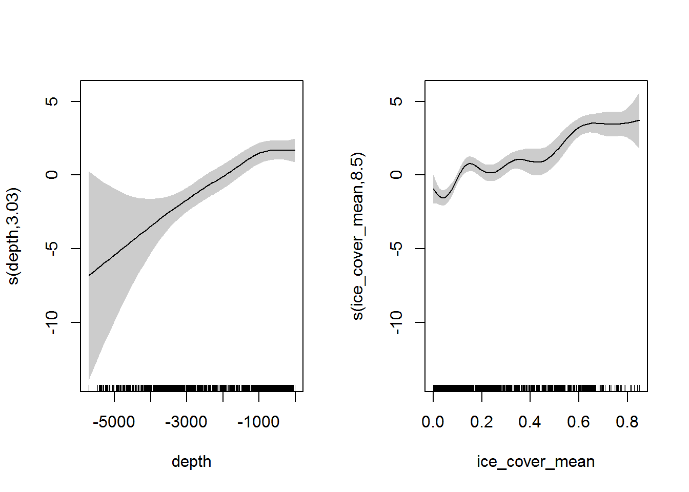

This suggests that we are more likely to find Euphausia crystallorophias in shallow areas with high annual ice cover, which seems plausible given that this species is typically found in coastal/shelf waters.

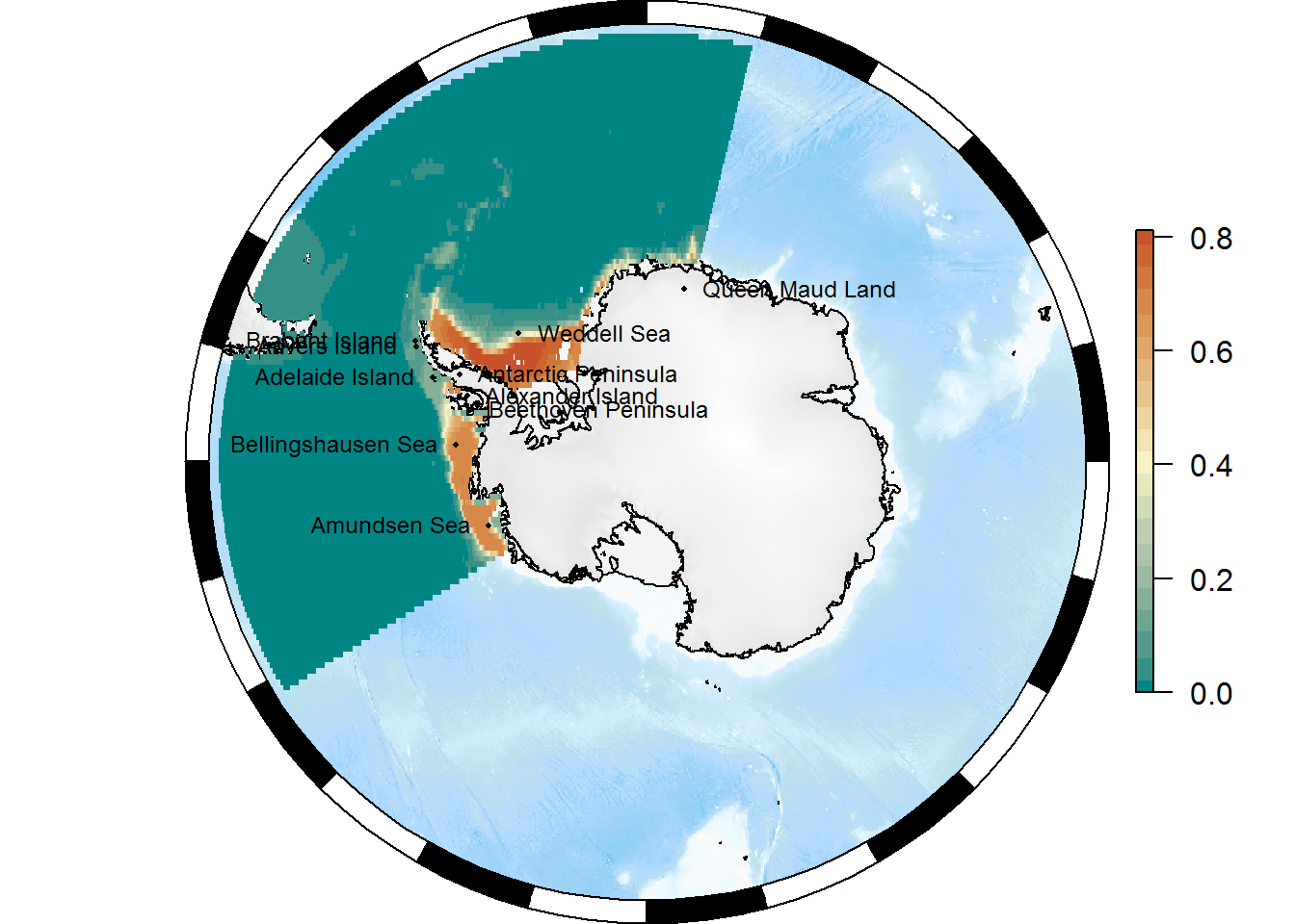
4.6 Predict from model

xpred <- expand.grid(lon = seq(from = floor(min(xfit$lon)), to = ceiling(max(xfit$lon)), by = 0.25),
                     lat = seq(from = floor(min(xfit$lat)), to = ceiling(max(xfit$lat)), by = 0.25))

xpred <- bind_cols(as.data.frame(xpred), as.data.frame(raster::extract(env_stack, xpred[, c("lon", "lat")])))

xpred$predicted <- predict(fit, newdata = xpred, type = "response")

## create raster
pr <- rasterFromXYZ(xpred[, c("lon", "lat", "predicted")])
projection(pr) <- "+proj=longlat +datum=WGS84"

my_cmap <- if (getRversion() >= "3.6") hcl.colors(21, "Geyser") else c("#008585", "#359087", "#539B8A", "#6DA590", "#85AF97", "#9BBAA0", "#AEC4AA", "#BED0B0", "#D0DCB5", "#E5E7BC", "#FBF2C4", "#F3E3B2", "#EDD59F", "#E7C68C", "#E3B77A", "#DEA868", "#DA9857", "#D58847", "#D1773A", "#CC6530", "#C7522B")

Plot it:

p <- SOmap_auto(x = pr, bathy = pr)
p$bathy_palette <- my_cmap
p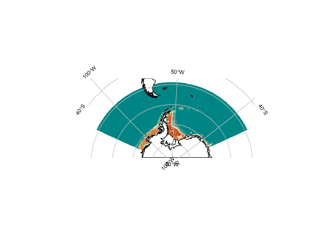

plot(basemap)
SOplot(pr, col = my_cmap)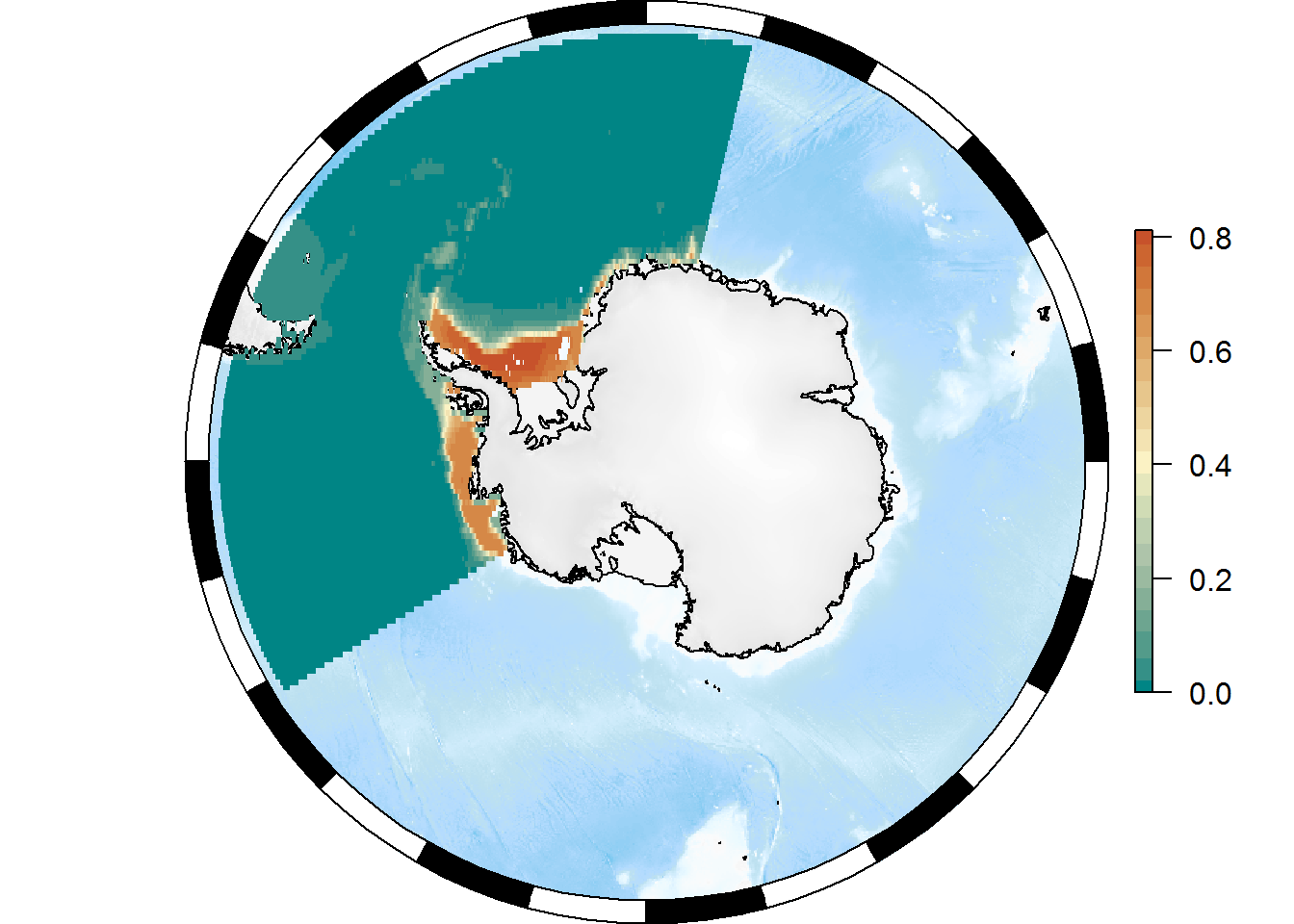

4.7 Other bits and pieces

4.7.1 Place names

library(antanym)

## The Composite Gazetteer of Antarctica is made available under a CC-BY license.
## If you use it, please cite it:
## Composite Gazetteer of Antarctica, Scientific Committee on Antarctic Research. GCMD Metadata (http://gcmd.nasa.gov/records/SCAR_Gazetteer.html)

## get full SCAR gazetteer data
xn <- an_read(cache = "session", sp = TRUE)

## reduce to one name per feature
xn <- an_preferred(xn, origin = "United Kingdom")

## ask for suggestions in our region to show on our map
xns <- an_suggest(xn, map_scale = 20e6, map_extent = extent(pr))

## transform to our map projection, convert to data frame, take the top 10
xns <- as_tibble(SOproj(xns, target = basemap$projection)) %>% head(10)

Add them to the map:

plot(basemap)
SOplot(pr, col = my_cmap)

## placename points
with(xns, points(x = longitude, y = latitude, pch = 16, cex = 0.4))
## and labels
with(xns, text(x = longitude, y = latitude, labels = place_name, 
               cex = 0.75, pos = 2 + 2*(seq_len(nrow(xns)) %% 2)))