Southen Ocean Diet and Energetics Data

Overview

This R package provides access to the SCAR Southern Ocean Diet and Energetics Database, and some tools for working with these data. For more information about the database see http://data.aad.gov.au/trophic/.

Installing

install.packages("devtools")
library(devtools)
install_github("SCAR/sohungry")

Usage

Basic usage: load the desired dataset using so_isotopes(), so_energetics(), so_lipids(), so_dna_diet(), or so_diet().

Examples

library(sohungry)
library(dplyr)
library(tidyr)
library(ggplot2)

Isotopes

Load the stable isotope data, in measurement-value format (one row per measurement):

xi <- so_isotopes(format = "mv")

Filter to taxon of interest, selecting d13C and d15N records:

xi %>% dplyr::filter(taxon_name == "Electrona carlsbergi" & measurement_name %in% c("delta_13C", "delta_15N"))

## # A tibble: 4 × 54
##   record_id source_id original_record_id     location     west  east south north
##       <dbl>     <dbl> <chr>                  <chr>       <dbl> <dbl> <dbl> <dbl>
## 1     1663.         8 Raymond et al. RECORD… Kerguelen …  71.2  72.2 -49.3 -49.1
## 2     1663.         8 Raymond et al. RECORD… Kerguelen …  71.2  72.2 -49.3 -49.1
## 3      483.        12 Raymond et al. RECORD… East of Ke…  70.3  70.3 -49.4 -49.4
## 4      483.        12 Raymond et al. RECORD… East of Ke…  70.3  70.3 -49.4 -49.4
## # … with 46 more variables: observation_date_start <date>,
## #   observation_date_end <date>, altitude_min <dbl>, altitude_max <dbl>,
## #   depth_min <dbl>, depth_max <dbl>, taxon_name <chr>,
## #   taxon_name_original <chr>, taxon_aphia_id <dbl>, taxon_worms_rank <chr>,
## #   taxon_worms_kingdom <chr>, taxon_worms_phylum <chr>,
## #   taxon_worms_class <chr>, taxon_worms_order <chr>, taxon_worms_family <chr>,
## #   taxon_worms_genus <chr>, taxon_group_soki <chr>, …

Diet

Load the diet data (stomach content analyses and similar):

x <- so_diet()

A summary of what Electrona carlsbergi eats:

x %>% filter_by_predator_name("Electrona carlsbergi") %>% diet_summary(summary_type = "prey")

Prey	N fraction diet by weight	Fraction diet by weight	N fraction occurrence	Fraction occurrence	N fraction diet by prey items	Fraction diet by prey items
Euphausia superba (Antarctic krill)	0		1	0.02	2	0.00
Amphipoda (amphipods)	1	0.01	0		0
Arthropoda (arthropods)	1	0.11	1	0.41	1	0.15
Chaetognatha (arrow worms)	1	0.10	0		1	0.33
Copepoda (copepods)	1	0.04	11	0.05	32	0.05
Euphausiids (other krill)	2	0.32	6	0.10	17	0.04
Fish	1	0.12	0		1	0.00
Gammaridea (gammarid amphipods)	1	0.04	1	0.20	1	0.25
Hyperiidea (hyperiid amphipods)	1	0.41	2	0.20	9	0.04
Salps	0		1	0.20	4	0.05
Uncategorized group	2	0.38	2	0.41	1	0.60

And what eats Electrona carlsbergi:

x %>% filter_by_prey_name("Electrona carlsbergi") %>% diet_summary(summary_type = "predators")

Predator	N fraction diet by weight	Fraction diet by weight	N fraction occurrence	Fraction occurrence	N fraction diet by prey items	Fraction diet by prey items
Aptenodytes patagonicus (king penguin)	1	0.07	10	0.24	2	0.00
Arctocephalus spp. (Antarctic and subantarctic fur seals)	19	0.00	35	0.05	15	0.03
Champsocephalus gunnari (mackerel icefish)	0		3	0.00	3	0.00
Dissostichus spp. (toothfish)	0		2	0.01	2	0.00
Eudyptes chrysocome (rockhopper penguin)	0		3	0.05	3	0.00
Eudyptes chrysolophus (Macaroni penguin)	0		1	0.06	0
Eudyptes schlegeli (royal penguin)	1	0.10	4	0.20	4	0.01
Mirounga leonina (southern elephant seals)	0		5	0.09	0
Pygoscelis papua (gentoo penguin)	1	0.28	3	0.18	1	0.49
Diomedeidae (albatrosses)	3	0.00	5	0.03	3	0.00
Ommastrephidae	0		1	0.15	0
Onychoteuthidae	1	0.07	1	0.15	1	0.04
Otariidae (eared seals)	0		1	0.04	0
Phalacrocoracidae (cormorants)	0		6	0.01	6	0.00
Procellariidae (procellariid seabirds)	13	0.01	29	0.08	23	0.00
Uncategorized group	1	0.02	1	0.05	1	0.00

Energetics

xe <- so_energetics()

Select all single-individual records of Electrona antarctica:

edx <- xe %>% dplyr::filter(taxon_sample_count == 1 & taxon_name == "Electrona antarctica")

## discard the dry-weight energy density values
edx <- edx %>% dplyr::filter(measurement_units != "kJ/gDW")

## some data manipulation
edx <- edx %>%
  ## remove the spaces from the measurement names, for convenience
  mutate(measurement_name = gsub("[[:space:]]+", "_", measurement_name)) %>%
  ## convert to wide format
  dplyr::select(source_id, taxon_sample_id, measurement_name, measurement_mean_value) %>%
  tidyr::spread(measurement_name, measurement_mean_value)

## what does this look like?
edx

## # A tibble: 248 × 8
##    source_id taxon_sample_id dry_weight energy_content standard_length
##        <dbl>           <dbl>      <dbl>          <dbl>           <dbl>
##  1        64              37    1.2               8.64              70
##  2        64              38    0.0067            5.34              15
##  3        64              39    0.00675           4.51              16
##  4        64              40    0.6               6.79              58
##  5        64              41    0.307             7.84              47
##  6        64              42    0.498             8.35              56
##  7        64              43    1.52              8.73              77
##  8        64              44    2.87              9.38              90
##  9        64              47    0.089             3.76              37
## 10        64              48    0.396             7.12              53
## # … with 238 more rows, and 3 more variables: total_length <dbl>,
## #   water_content <dbl>, wet_weight <dbl>

Plot the wet weight against wet-weight energy density:

p <- ggplot(edx, aes(wet_weight, energy_content))+geom_point()+theme_bw()+
  labs(x = "Wet weight (g)", y = "Energy density (kJ/g wet weight)")
plot(p)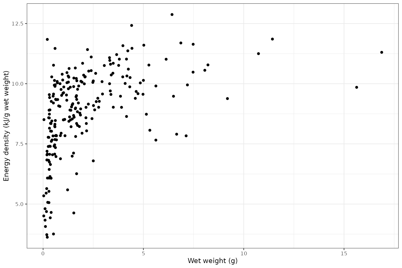

Fit an allometric equation:

fit <- lm(log(energy_content)~log(wet_weight), data = edx)
px <- tibble(wet_weight = seq(from = min(edx$wet_weight), to = max(edx$wet_weight), length.out = 51))
px$energy_content <- exp(predict(fit, newdata = px))
p+geom_path(data = px, colour = "dodgerblue")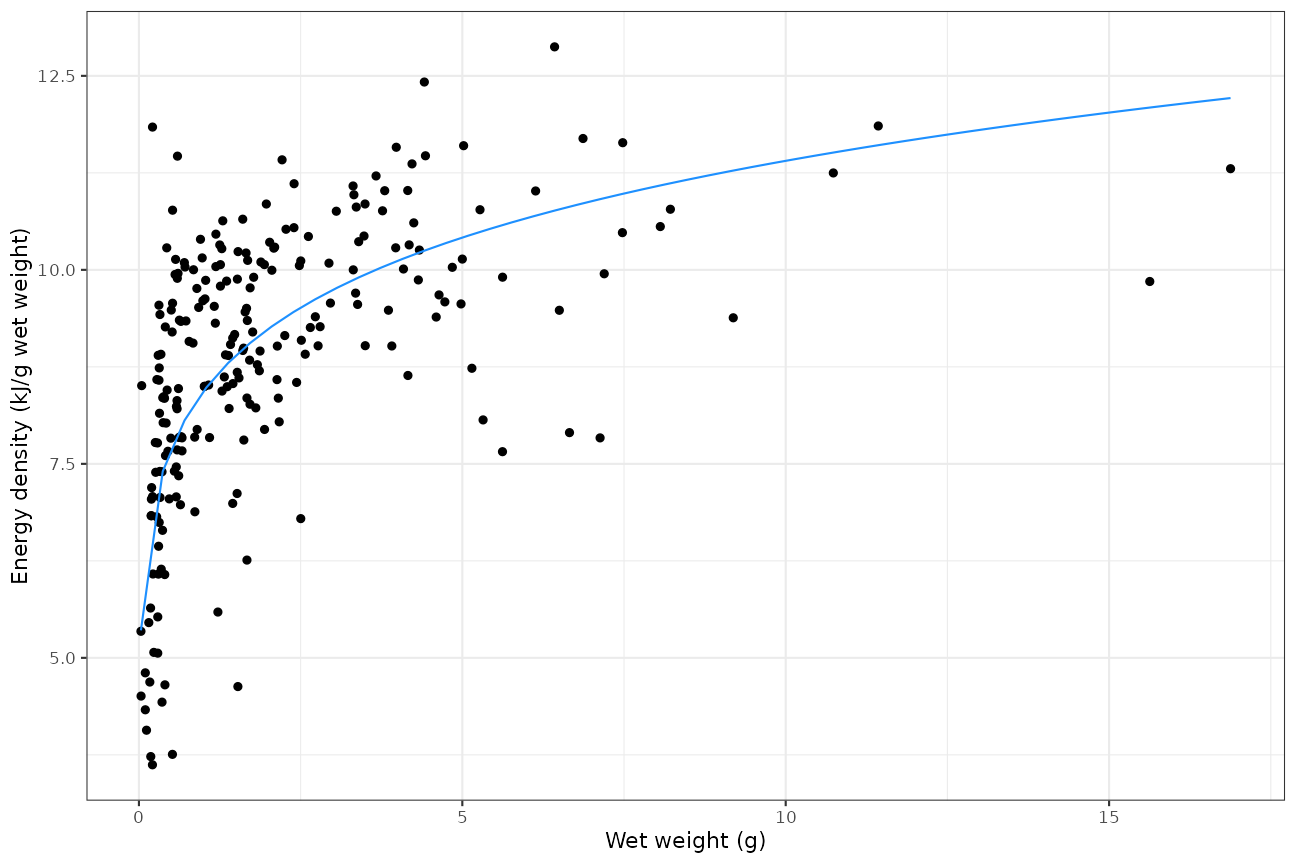

Lipids and fatty acids

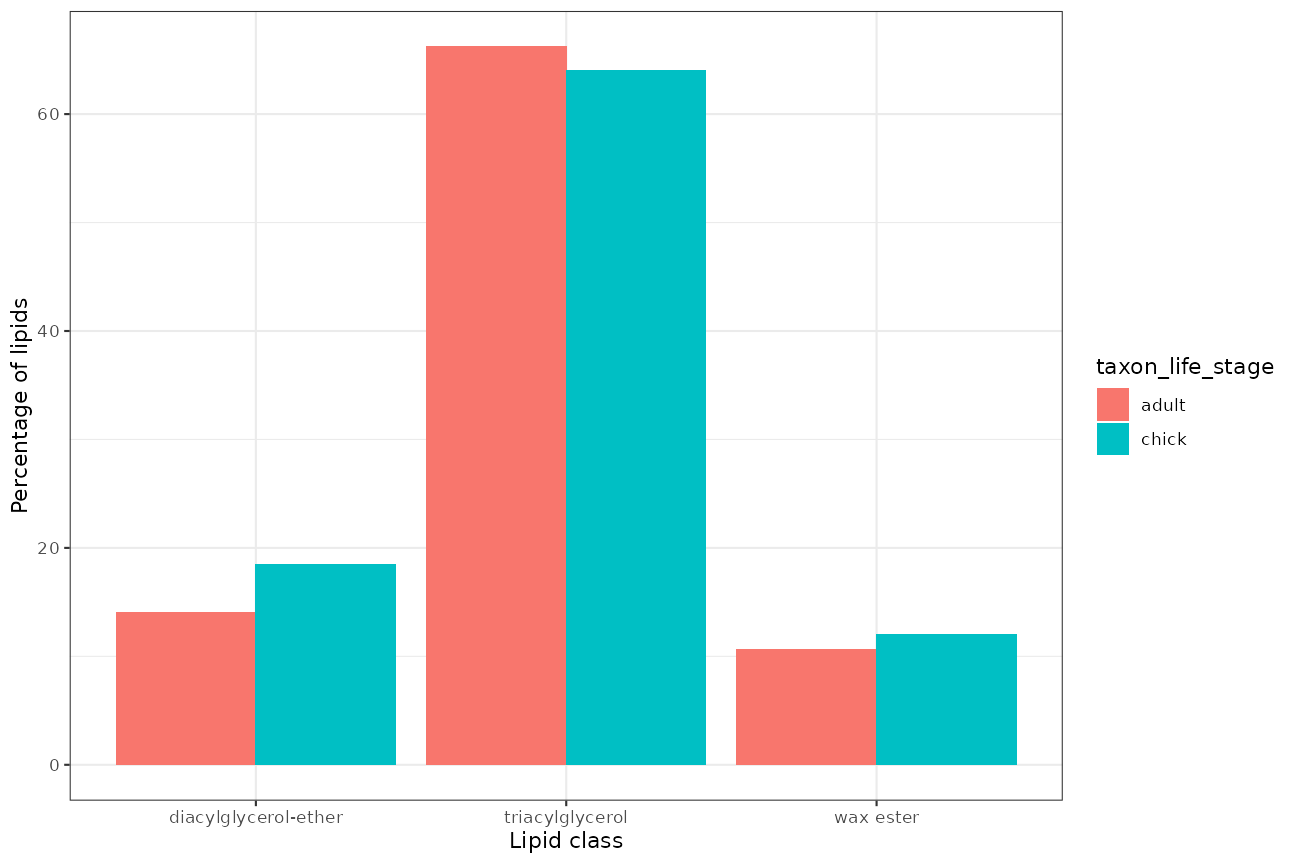
xl <- so_lipids()

Select lipid-class data from Connan et al. (2007), and plot similar to Figure 2 from that paper:

xl <- xl %>% dplyr::filter(source_id == 126 & measurement_class == "lipid class") %>%
  mutate(measurement_name = sub(" content", "", measurement_name)) ## tidy the names a little

ggplot(xl,
  aes(measurement_name, measurement_mean_value, fill = taxon_life_stage, group = taxon_life_stage))+
  geom_col(position = "dodge")+theme_bw()+
  labs(x = "Lipid class", y = "Percentage of lipids")

Ben Raymond

2021-11-18